Home About us Contact us Training Optimisation Services Protuner Educational PDFs Loop Signatures Case Histories
Michael Brown Control Engineering CC
Practical Process Control Training & Loop Optimisation
HAVING FUN WITH A POSITIVE LEAD ON AN INTEGRATING PROCESS
One of the most interesting dynamics that can be found in the industrial control world is what is known as a first order lead on an integrating process.
A positive lead integrator responds to a step change with a kick followed by a typical integrator ramp. It is commonly found on back pressure control of steam dryers on paper machines, on density controls in mining applications, and also on certain temperature processes. However this strange phenomenon also appears from time to time on processes, often where one least expects it.
Positive lead integrators are probably the most interesting of all the different dynamics you will ever come across, and normally the most rewarding, as you can often achieve spectacular improvements in loop performances when you tune them. Most loops that one encounters with these dynamics are usually terribly poorly tuned, with most of them reacting extremely slowly to changes. In some cases, correct tuning can improve response by several thousand times! Really dramatic stuff!
The problem with this type of dynamics is that very few people recognise it or have received training on how to deal with it. Like all process dynamics that incorporate leads, incorrect tuning can quickly result in instability. Operators are normally terrified of responses with leads as they tend to give a big kick, and they think the process is “running away”.
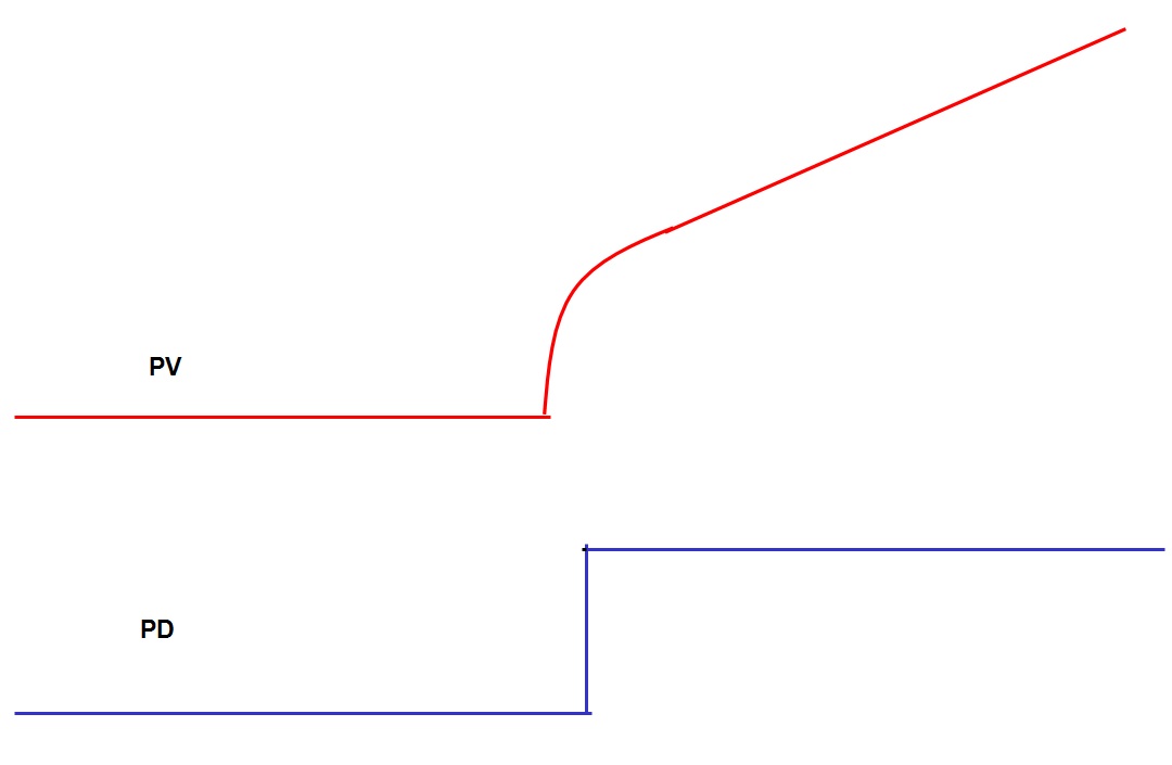
A full description, the transfer function, and explanation of how to deal with positive lead integrators is given in my Loop Signature articles LSp2-20 and LSp2-21. However in brief, the change to a step change on the output of the controller with the controller in manual results in an initial rapid rise of the PV (process variable) followed by the slower integrating ramp. This can be seen clearly in Figure 1.
Figure 1.
In actual fact a first order lead on an integrating process actually consists of two things. The first part of the response (the lead) is actually the typical response of a common first order lag, dead time, self-regulating process, similar to a flow process, which then turns into a simple integrating process, , similar to a level process.
It sounds complicated, but it’s not. The following example will show why, which is taken from some work I did recently at a chemical plant.
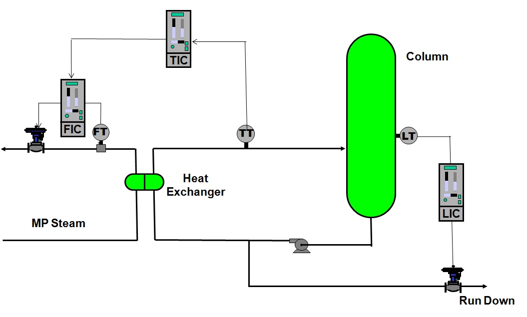
Figure 2.
The particular process is the reboiler control loop on a distillation column. Figure 2 shows some of the controls on the column. Fluid is pumped from the bottom of the column and reheated through the heat exchanger from where it is fed back into the column. Basically the purpose of the temperature controller shown in the figure is to keep the temperature constant on the output of the heat exchanger. This is done by adjusting the flow of medium pressure steam passing through the other side of the heat exchanger. As can be seen the flow is actually controlled by a secondary cascade flow control loop, the setpoint of which comes from the output of the temperature controller.
I have written a lot about cascade loops in other articles, but to recap, it is in my opinion an essential control strategy that should always be employed when trying to control important slow loops like temperature and levels, to name but a few. The reason for this is that the secondary flow loop acts very much faster than the slow primary loop, and thus ensures that the correct flow is put into the process to satisfy the control requirements as demanded by the slow primary controller. To put it even more simply: It eliminates problems such as steam pressure variations, valve hysteresis, valve stickiness, and installed valve non-linearities.
The purpose of the level control loop is to keep the bottom level in the exchanger constant, and thus the volume of the pool of liquid in the bottom of the exchanger is kept constant.
Back to our positive lead effect: In this particular case the heat exchanger has an extremely fast reaction to changes in steam flow. So if one was to make a step change on the steam flow with the temperature controller in manual there will be an initial fast rise of temperature of the fluid going through the exchanger which then passes into the column. This is the initial self-regulating effect. This hotter fluid will in turn slowly start increasing the temperature of the liquid pool in the bottom of the column, which is then passed back into the heat exchanger. As time goes by, and as the liquid circulates round and round, the temperature of this pool will increase in a ramp fashion. This is the integrating effect. Thus one can now see how the overall dynamic response is initially self-regulating, but then becomes integrating.
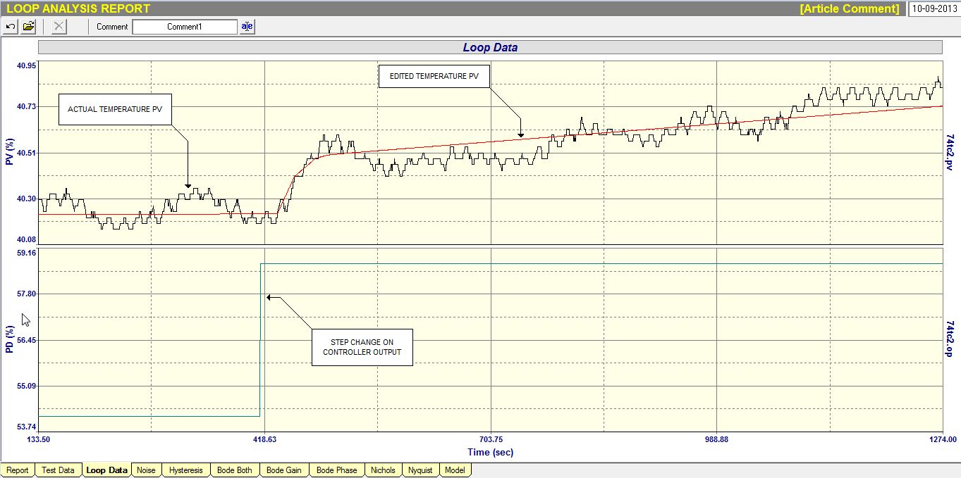
Figure 3.
The actual open loop test performed on the temperature control loop is shown in Figure 3, where a step change was made on the output of the controller. When one performs these tests you have to be very careful to keep the steps as small as possible so as to avoid upsetting the process too much. Large upsets can damage product quality, and possibly also upset downstream columns, and thus create huge production problems. In actual fact the change of temperature as shown in the test moved the temperature only by an incredibly tiny 0.9ºC (which is about 0.6% of the actual temperature range)! This why the temperature PV trace appears to be so “noisy”. One cannot even see the variations on a 0-100% scaling.)
Even the Protuner would not be able to give good tuning with these “noisy” fluctuations in the PV, so one has to perform a graphic edit, to produce the true response. This is shown on the red line in the figure, and the tuning is performed on the edited PV.
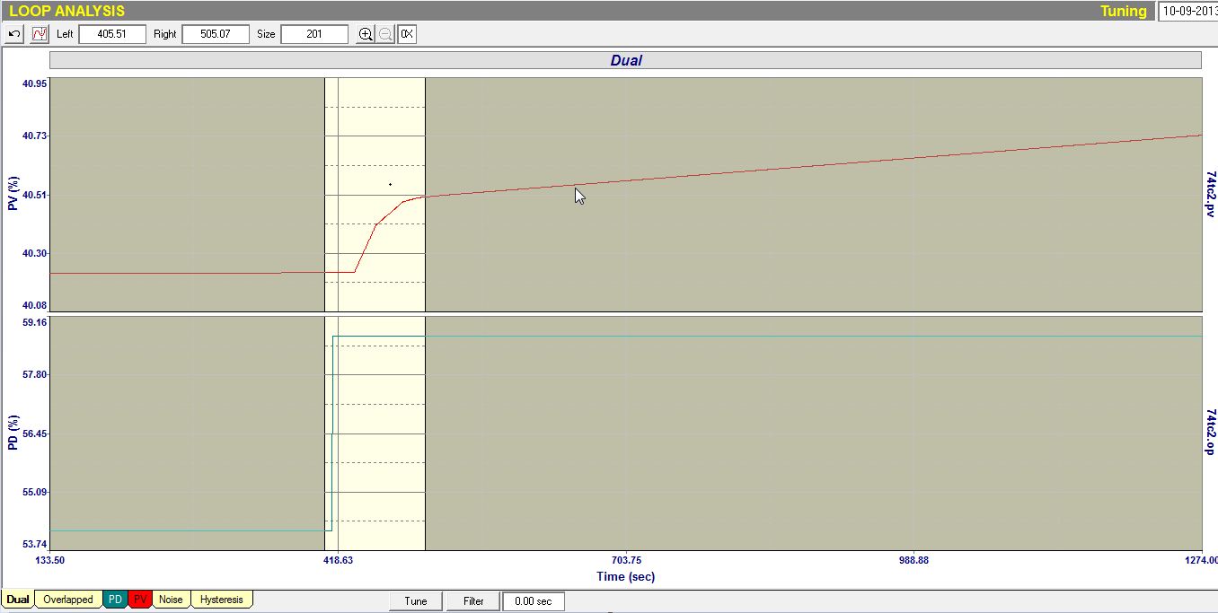
Now the magic of tuning a first order positive lead on an integrator, is that you tune on the initial self-regulating response i.e. the lead portion, and completely ignore the integrating part. This is done by windowing the self-regulating part of the response as shown in Figure 4, and tuning in that window. If you tune over the whole response, as most people do, then one gets an incredibly slow tune.
Figure4
This is borne out by the difference of the as-found, and final tuning on this loop:
The as-found tuning: P = 5.0, and I = 10.5 minutes/repeat.
The Protuner correct final tuning: P = 3.0, and I = 0.3 minutes/repeat.
This tuning is probably a hundred times faster than the original, and worked incredibly well, keeping the temperature at setpoint within a band of ±0.1ºC under conditions of quite severe load changes. The people on site get very excited when they see how well this tuning works. I often refer to it as a lovely “party trick”.
Just out of interest I have optimised many reboiler temperature controls on distillation columns but in most cases there are no leads, and the process is usually purely integrating. The reason that this one had such a prominent lead is due to the fact that the heat exchanger has as extremely fast response. One could say that it is probably oversized, although this is good as it allows much faster temperature control.