Home About us Contact us Protuner Loop Analyser & Tuner Educational PDFs Loop Signatures Case Histories
Michael Brown Control Engineering CC
Practical Process Control Training & Loop Optimisation
LOOP SIGNATURE 15
DIGITAL CONTROLLERS PART 7
THE D TERM (THE FINAL PART)
This last article on the subject of derivative will deal with choosing the right response in the controller if you wish the derivative action to work on setpoint changes as well as on load changes. (A load change can be defined as a change in the PV value caused by external effects on the loop, and not caused by movement in the output of the controller).
Figure 1.
A schematic of a simplified PID controller with a parallel algorithm is shown in Figure 1. Either a step change in setpoint, or a step load change in the opposite direction, will both result in an identical step change in error. The error is then fed in parallel to the P, the I, and the D block. The response of each is shown in the diagram. These are then arithmetically added together and converted to a 4 - 20 mA current signal, which is the output of the controller (or process demand signal). As can be seen, the final result would cause the valve to kick open, and then back quite sharply, and this would then be followed by the normal integral response.
This is not a desirable response in most processes. To understand this we must look at the average process where PID controllers are employed. The vast majority of controllers are used in continuous type process plants typified by petrochemical, chemical, paper, and other similar plants. Generally these plants have multiple processes where one process feeds the next, and so on down the line. The plants are often complex and difficult to start up. Once up and running, the object is to try and optimise them for maximum productivity, and then to keep them running in this state as smoothly as possible, and for as long as possible. If a valve, particularly near the beginning of the plant was to react as seen in Figure 1 when the plant is running steady state, then it is highly possible that everything downstream would react to the kick and cause considerable disruption to production, even to the extent of causing a trip.
This gives rise to the popular belief that controllers are better detuned in continuous process plants to prevent "bumps". Many people are very unclear on this point. The author when about to optimise a loop, has been frequently told that the loop is critical to the plant performance and needs to really perform well, but on the other hand it must not be tuned fast so as to cause a downstream disturbance. (Talk about diametrically opposed requirements). We do in practice find that the vast majority of loops in such plants are completely and utterly detuned. However when we go into these plants we get told:
"Our controls are great. 99% of our controllers are in automatic and if you look at the trends, you will find they are all running on setpoint."
What actually occurs in reality under steady state conditions is that generally for the vast majority of the time no changes are occurring. Therefore the controllers are not doing anything. In particular on self-regulating processes, if you tune a controller however slowly and put in some gain and a little integral, it will eventually get itself to setpoint.
This all sounds reasonable. So why do we even bother putting in controllers? David Ender of Techmation Inc. of the USA who is a world leading experts in loop optimisation, has defined the purpose of the regulatory control system as "minimising control variance at all stages of production".
Control variance may be thought of very roughly as total integrated control error. The controllers are there to keep the process on setpoint as closely as possible under changing conditions. This is not going to be achieved if the controllers are detuned. Therefore we find that continuous process plants, whilst working well for a lot of the time, start swinging badly if conditions start changing. An excellent example of this is in plants that are exposed to atmospheric conditions like petro-chemical refineries. They are operating fine, and suddenly a rainstorm or a cold front hits them. The next minute everything starts drifting off. The controllers are so detuned they cannot respond quickly enough. The operators put loops into manual to try and catch the load changes, and it may take hours to get things back to optimum.
Therefore to prevent this, what is needed to minimise control variance is in fact controllers that respond really quickly to load changes. Going back to the problem of the derivative kick, one must look at the difference between load changes on such plants and setpoint changes. Load changes in a continuous process plants are seldom step changes. Normally one finds the process variable drifting off from setpoint in a slow ramp fashion. We would like to correct this as quickly as possible, and if we use derivative on a process, it will not respond to the ramp with a big kick but with a little step. On process types where derivative is effective, you will get the process back to setpoint much quicker with it.
Setpoint changes on the other hand, are normally step changes. Why would one need to make setpoint changes under steady state operating conditions? The answer is that even when the plant is running steady, the operators often make small changes to optimise processes. The large derivative kick then is a problem as it occurs irrespective of the size of the step change. It is also apparent that fast response to setpoint changes is generally not needed.
Therefore we can in general propose that the controllers should respond slowly to setpoint changes, and quickly to load changes.
When the electronic controllers were introduced in the 1960's, their designers looked at this, and came up with two solutions. The first was to allow the user to put ramps on setpoint changes. This is still available on most controllers, although it is seldom used. The second option was to reconfigure the controllers to eliminate the derivative action on setpoint changes, whilst still allowing it to act on load changes.
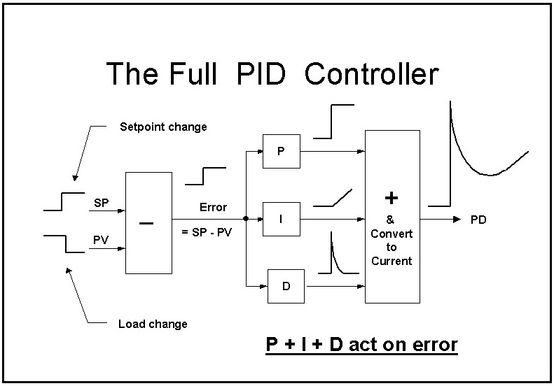
Figure 3.
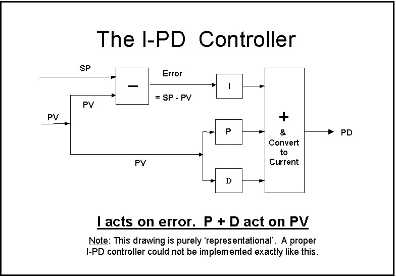
Figure 3 shows another popular configuration of controllers, the I-PD controller, where now both P and D are on the PV, and only the I on the error. (Please note that as mentioned in the diagram, the drawing is only representational only. The P action does in fact have to respond to the magnitude of the error, even if it only does so on PV change). This configuration gives the least bump of all on setpoint change, as the integral action is always a ramp.
People often question if the I-PD controller has any real worth. The answer is yes. There are many applications, particularly on level control, where one has high proportional gain in the controller, and setpoint changes should not bump the valve too much, although fast control is required for load changes. There are a lot of applications like this in petro-chemical refineries and paper plants.
It should be noted that this controller configuration is untunable. At the very least, it is essential that one can see how the proportional action reacts to setpoint changes. Fortunately most manufacturers (but not all) that supply the I-PD controller (generally as their default controller), allow one to change it to at least a PI-D configuration. The manufacturers probably did this, not with the thought of tuning in mind, but did realise that the secondary controller in a cascade control system could not operate properly without at least the P action.
In conclusion we can summarise the various points discussed on derivative as follows:
* Derivative is only useful on slow self regulating processes with multiple first order lags, and integrating processes with a large lag.
* The derivative filter should be placed before the derivative block only, and the value of its coefficient should be between 0.125 and 0.25.
* A controller should be configurable to allow one to choose all three actions on setpoint change, viz. PID, PI-D, and I-PD.
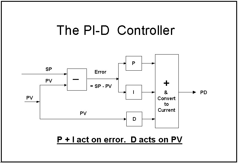
Figure 2 shows such a configuration. The D block has been removed from the error signal, and the PV is now its input. Thus on a setpoint change there is no initial derivative action, only P+I, whilst on a load change, the error causes the P+I to react, and the PV causes the D to act, resulting in a full P+I+D action. Some manufacturers sometimes refer to this configuration as "PI-D" control action.
The vast majority of controllers are supplied with this as their default configuration. Indeed most manufacturers do not even allow you to configure a controller with P+I+D on error. The PI-D configuration is of extreme interest from the practical point of view, for how can we tune in the D term on such controllers? Even if you have the world's greatest tuning package, generally the only way to actually test how the derivative action is performing is to make a setpoint change. If your controller does not respond with D to a setpoint change when performing tuning, then you have a major problem, as you cannot judge if the D term has been set correctly.
The only way one can perform such tests now is to make step changes in load. This is not easy to do, and generally the process people are violently opposed to doing this. Bearing in mind that the vast majority of all tuning is done by trial and error (or "playing with the knobs", whilst making setpoint changes), this is the last and probably the main reason why derivative is hardly ever used in real life. Once again it illustrates the lack of knowledge of practical control displayed by manufacturers of controllers. It is the author's firm belief that no one should ever purchase PID controllers where the user cannot configure a full PID action on error so that derivative can be tuned and tested.
It is not only for tuning that one would require a full PID action on setpoint change. Certain processes like temperature batch reactors need to respond as fast as possible to setpoint changes.