Michael Brown Control Engineering

Home About us Contact us Training Optimisation Services Protuner Educational PDFs Loop Signatures Case Histories

Michael Brown Control Engineering CC

Practical Process Control Training & Loop Optimisation

LOOP SIGNATURE 21

YOU CANNOT CONTROL IF YOUR MEASUREMENT IS INCORRECT

The first law of process control could be stated as saying that you cannot control if your measurement is incorrect. I use this as a slide in my courses. On one occasion a delegate protested that I was really insulting the class’s intelligence by putting up a slide with such an obvious statement.

Certainly I have no intention of insulting anyone. We all know this law. However do we all remember it in the “heat of the moment”?
My experience is that most instrument technicians with “gut feelings” developed over years of uncertainty in the practicalities of process control, will try and solve all problems by playing with the magic tuning knobs, P, I, and D. Also if anything goes wrong in the plant, the first thing the process people do is to blame the control system, and ask for someone to come and retune the controller. In our courses we try and teach people that tuning is the last thing one should touch.

Many people also seem to place tremendous reliance in their measuring instruments, especially if these are “smart” (i.e. computerised). Another of the great fallacies in control is that “computers can overcome all problems”. Some people even seem to believe that computers can override natural laws of physics. To site an example I was in a petro-chemical refinery where they were having trouble on a flow loop using an orifice plate and differential pressure transmitter as the measuring system. They were trying to control the flow at 10%. When I told them that you couldn’t use an orifice plate type measurement at such a low point in the range, one of their advanced control engineers took issue and said to me that there shouldn’t be a problem as they were using a smart transmitter with a square root extractor in it. He had forgotten all his basics of the principles of such a measurement. Even a computer cannot get around these laws, and generally one should never work with a flow below 25% minimum with such a measuring system. (Before I get a flood of letters back from angry suppliers, I am aware that there are now some few and very special transmitters that now let you get an 8:1 rangeability on orifice plate measurements. However the transmitter in this particular case was not one of these.)

One of the other things I have become very aware of in plants is that many instrument people seem to rely entirely on the supplier for setting up a measuring system. Very often the plant people do not seem to understand very much about the instrument, how it works, its specifications, its limitations, and other important things. Many times I have asked people to get out a particular manual, only to be told that there isn’t one, or else they can’t find it. On one occasion we did get the manual, and on opening it I discovered there were 18 user adjustments, most of which I couldn’t understand. However there wasn’t a single person in the plant (which had a lot of instrument people) who had even read the manual, or who knew anything about the calibration of the instrument. I believe it essential that if you are reliant on a measurement for good control, you should satisfy yourself that you are fully familiar with, and understand all the various “ins and outs” of the device to ensure that you yourself are satisfied the measurement is correct.

Figure 1.

There are a few points I would like to discuss concerning the use of smart transmitters that I find many people are unaware of.
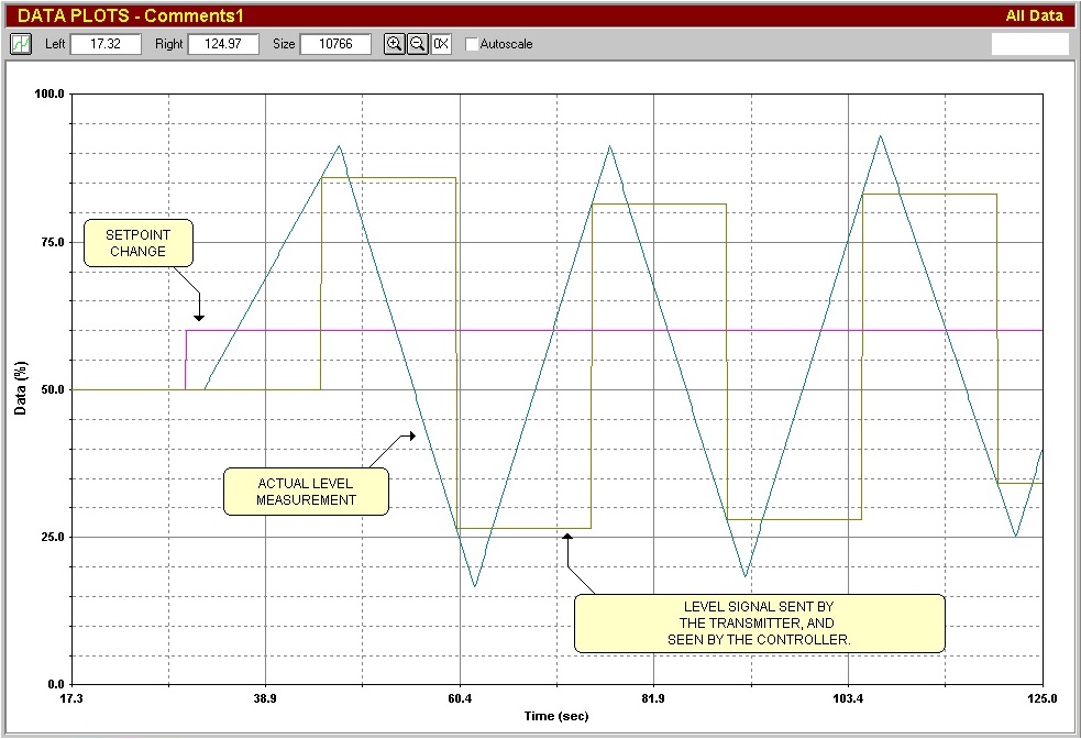
Firstly the scan rate (output update repetition rate) of the device should be fast enough to follow process changes to allow the controller to react correctly. It must be remembered that the controller acts on the signal received from the transmitter. So if we have a process that can change very quickly, and if the transmitter does not scan quickly enough to send changes to the controller, then instability can result.

An example of this was at a mining plant where the operators could manually control the level in a fast flotation tank. As soon as they put it into automatic it went unstable. On investigating the loop it was found that the ultrasonic level transmitter had a scan rate of some 15 seconds. During this period the level could move quite a few percent. As a result, the controller, which was scanning every half a second, was receiving out of date information. This resulted in an unstable cycle, as illustrated in Figure 1. In the figure one can see the true level being sampled by the transmitter every 15 seconds. This resulted in the controller taking violent action on every new scan correct the error, and causing the valve to reverse.

The next point is that with today’s computerised systems we may have several computerised devices passing information along the line. For example you may be feeding a signal from a smart transmitter to a PLC. The smart transmitter has a scan rate. The PLC may have a set of analogue input cards with their own scan rate. Then the controller in the PLC will also have its own individual scan rate.

It is a generally accepted law that digital devices should sample at a rate at least twice as fast as the next downstream digital device, or instability can occur, (provided their scans are not simultaneously synchronised). A general rule of thumb is that the upstream device should be at least five times faster than the downstream one. Once again the reason behind this is to prevent the controller receiving “out of date” information.

In reality neither of the above two points will affect one if the process is slow. However there is no doubt that instability can occur in fast processes.

Figure 2.

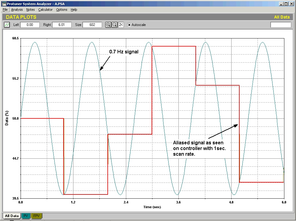
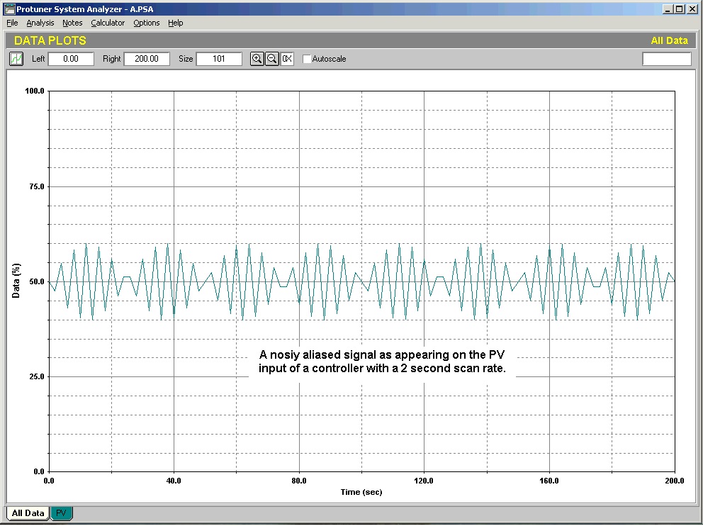
Aliased signals may contain many lower frequency harmonics, and cause strange things to happen. Figure 3 illustrates how a signal with a strong sinusoidal component of 0.7Hz will be aliased by a controller with a scan rate of 2 seconds. Note that there are some really low frequency components in the alias. A control loop in automatic can easily start responding to these elements, and can actually cause a loop to oscillate as if it was unstable.

Figure 3.

Figure 4.

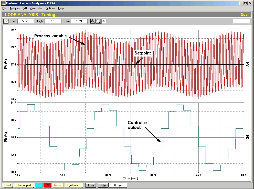
This is illustrated in Figure 4, which shows a recording of a loop running in automatic, which is cycling. The instability is caused by the loop following a low frequency sinusoidal component caused by a signal alias. The tuning is in fact very stable.

This article has stressed how important it is to ensure that measurements are correct. People so often ignore this. During the course of writing this article, a classic example of the apparent refusal to believe measurements can be wrong occurred at a paper plant where I was optimising the controls on a paper machine. One of the most critical loops on the machine, the basis weight control, was behaving badly and fluctuating around badly on an intermittent basis, literally once or twice a shift for about an hour. Analysis revealed that the problem was occurring because the flow measurement was fluctuating badly, on this intermittent basis. It is very easy to prove that it was not the control causing it by merely placing the controller in manual. The fluctuations could in fact have been due to actual flow fluctuations, or due to a problem in the magnetic flow meter. (At time of writing this, the cause had not been resolved, but it would appear likely to be the flow meter, as other process variables which would have been affected by actual flow fluctuations remained steady). The fluctuations were so bad that in automatic control they caused the valve to swing around far too much, badly affecting control variance. I explained to the Operators that until the I&C department could sort the problem out, that when these fluctuations were occurring, they should run the loop on manual until they disappeared again.

They refused to believe all this. As far as they were concerned we had been working on the system doing tuning, and it must have been something we had done - even though they had experienced the same problem before we started on the plant. Although I spent time with them explaining the findings, they complained to various supervisors, and they changed tuning parameters themselves overnight. (Another new mystery: How did they get through the security codes to change tuning parameters?).

Eventually the Production Manager came storming down “to sort us out”. Fortunately once I could calm him down and explain things to him, he did fully understand, and got everyone else to cooperate, until the problem could be solved. (The first step was that a new magnetic flowmeter was going to be installed on the next plant shutdown).

To me this once again illustrates a point I am always stressing, both in these articles, and in my courses. It is essential for both process and I&C people to work as a team when performing optimisation. One of my first requests when optimising a plant is for someone with a really excellent knowledge of the process to be assigned to work with me. Unfortunately, these people are rare, have heavy workloads, and demands on them, and as a result it is very seldom that I actually get my request granted. If it was the optimisation would probably be more successful, take less time, cause less disruption to production, would break down parochial barriers, and would get the process people to happily accept, and actually welcome properly optimised control systems.

Figure 3.

Figure 4.