Home About us Contact us Protuner Loop Analyser & Tuner Educational PDFs Loop Signatures Case Histories
Michael Brown Control Engineering CC
Practical Process Control Training & Loop Optimisation
Loop Problem Signatures Part 2 - 14
DYNAMICS OF SIMPLER PROCESSES
Negative Lead-Lag, Deadtime, self-regulating process
The transfer function of this process is:
Where:
PG = process gain
-L = Negative lead in seconds.
TC = Lag time constant in seconds.
DT = deadtime in seconds.
s = Laplace operator.
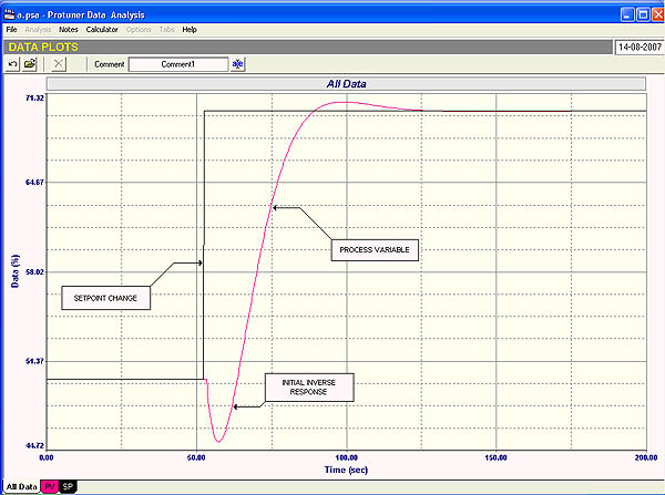
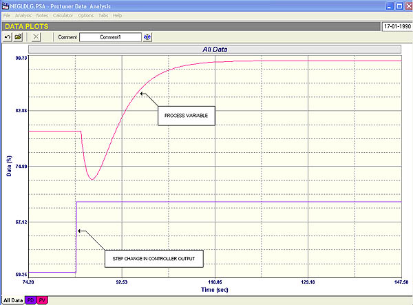
The response to an open loop step change is shown in Figure 1.
Fig. 1
One is very unlikely to encounter such a response in actual practice. The only time I personally ever saw a response like this was on a flow loop where there was insufficient air supply pressure to the valve and positioner. When one made a step change on the controller output, the pressure initially “collapsed” and the valve actually started moving the wrong way until sufficient air pressure could build up to send it in the right direction. The solution to this problem is obviously to fix the air supply, so the valve operates correctly, and not to try and sort out the problem by tuning.
I have been told that the response is sometimes to be found on the temperature control of a distillation column when a step change is made on the flow coming back in from the reboiler. This affects the vapour balance in the column and caused an initial change in temperature in the inverse direction before it recovers and moves the right way. However I have personally tuned quite a few of these loops and have not encountered this. This does not mean that I will not encounter it on another distillation column I may “meet” in the future.
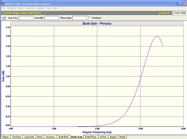
Fig. 2
Figure 2 shows the Bode Open Loop Gain Plot of the process. It should be noted how the right hand side of the plot has been pushed upwards. This is due to the lead, which has this effect on the plot. (This is also similar to the plot we saw for the second order lag shown in the last loop Signature article in this series.) Once again this means that the controller gain must be severely cut back to bring the right hand side of the plot down to achieve sufficient gain margin, which of course will result in fairly slow control.
Another point to note again is that the derivative term must never be employed on this type of process, as the last thing one would like is to push up the right hand side of the plot even further.
Another way of looking at it is to think of the inverse part of the response as being like deadtime. The controller must not react too quickly whilst the process is going “the wrong way”.
In general negative leads are really a bad thing. Apart from just having to slow the control, a major problem can arise when an inverse response occurs on a load disturbance. In this case even though the feedback controller is tuned to react slowly, it will also initially react incorrectly when the load disturbance occurs, as it sees the process start moving in a particular direction. It will try to correct it immediately and push its output to try and reverse the process movement. This in fact moves the valve in the wrong direction and will immediately induce a second inverse response, which will add to the one initially caused by the load change. This effectively doubles the inverse movement, and this then has to be corrected by the controller once the process reverses and starts moving in the correct direction. This can lead to huge deviations from setpoint, and in certain cases can even result in a plant trip.
It will be shown later in this series, that one good solution is to employ feedforward control.
The process with the open loop response shown in Figure 1 has the following various dynamic constants:
PG = 1
L = -8 seconds.
TC1 = 5 seconds.
TC2 = 2seconds. (There is often a small second lag in this type of response).
DT = deadtime in seconds.
The controller was tuned with a proportional gain of 0.2 and an integral of 4.1 seconds/repeat.
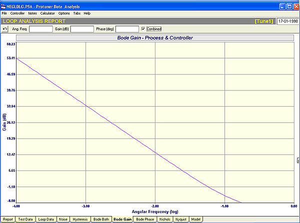
Fig.3
The combined (closed loop) Bode Gain Plot with this tuning is given in Figure 3. It can be seen that the pole cancellation is not wonderful and the plot is bent up at the bottom instead of sloping down the whole way at ‑20db/decade, which is the ideal. However it is the best that can be done here. It will be remembered from a previous article in this series that such a plot with the bottom bent upwards results is control slower than desirable, and it may have a tendency to “step-up” to setpoint.
Fig. 4
The closed loop response to a step change in setpoint is shown in Figure 4.
It will also be shown later in this series that positive leads are normally much easier to deal with than negative leads. (They can be cancelled out by inserting an additional lag in the loop). Unfortunately there is nothing one can do to cancel negative leads, if they do occur, but one can sometimes try and minimise them by better process design.